Single fidelity surrogates

Surrogates is one of the most important part in the multi-fidelity optimization. In this module, we implement the surrogates for single fidelity and multi fidelity. For single fidelity, we implement the following surrogates:

Kriging model

Kriging model is a Gaussian process regression model with a constant mean function and a squared exponential kernel. The Kriging model is implemented in GaussianProcessRegression class.

1. basics of Kriging model

A Gaussian process if completely specified by its mean function and alert{correlation} function, which can be defined as:

\[m(\mathbf{x}) = \mathbb{E}\left [ f \left( \mathbf{x} \right) \right]\]

\[k(\mathbf{x}, \mathbf{x}') = \mathbb{E}\left [ (f (\mathbf{x}) - m(\mathbf{x}) )(f(\mathbf{x}') - m(\mathbf{x}'))\right]\]

Therefore, Gaussian process can be write as:

\[f(\mathbf{x}) \sim \mathcal{GP} (m(\mathrm{x}), k(\mathrm{x}, \mathrm{x}'))\]

Usually, the RBF kernel function is defined as:

\[k(\mathrm{x}^{i}, \mathrm{x}^{j}) = exp\left(-\sum_{d=1}^{k} \theta_d \left({x}_{d}^{i}-{x}_{d}^{j}\right)^{p_d}\right)\]

where \(k\) is the dimension of the problem, \(\mathrm{\theta}\) and \(\mathrm{p}\) are two \(k\)-dimensional vectors of hyper-parameter The correlation matrix is defined as:

\[\begin{split}\mathrm{K}(\mathrm{X,X}) = \begin{bmatrix} k(\mathrm{x}^{1}, \mathrm{x}^{1}) & ... & k(\mathrm{x}^{1}, \mathrm{x}^{n})\\ ... & ... & ...\\ k(\mathrm{x}^{n}, \mathrm{x}^{1})& ...& k(\mathrm{x}^{n}, \mathrm{x}^{n}) \end{bmatrix}\end{split}\]

where \(n\) is the number of samples

2. Negative log-likelihood

The negative log-likelihood of the Gaussian process is defined as:

\[\ln(L) =-\frac{n}{2}\ln(2\pi) - \frac{n}{2}\ln(\sigma_e^2) - \frac{1}{2}\ln|\mathbf{K}| -\frac{(\mathbf{y}-\mathbf{1}\mu)^T\mathbf{K}^{-1}(\mathbf{y}-\mathbf{1}\mu)}{2\sigma_e^2}\]

in which, \(\mathbf{y}\) is the vector of observations, \(\mathbf{1}\) is a vector of ones, \(\mu\) is the mean function, \(\sigma_e^2\) is the variance of the noise, \(\mathbf{K}\) is the correlation matrix. Overall, it has 2n + 2 parameters to be optimized, furthermore, the hyper-parameters can be estimated with the following two steps:

1. step 1: take derivative of the negative log-likelihood with respect to the hyper-parameters \(\mu\) and \(\sigma_e^2\) and set them to zero, we can get the following equations:

\[\hat{\mu} = \frac{\mathbf{1}^T\mathbf{K}^{-1}\mathbf{y}}{\mathbf{1}^T\mathbf{K}^{-1}\mathbf{1}}, \,\, \hat{\sigma_e}^2 =\frac{(\mathbf{y}-\mathbf{1}\mu)^T\mathbf{K}^{-1}(\mathbf{y}-\mathbf{1}\mu)}{n}\]

2. step 2: substitute the estimated hyper-parameters into the negative log-likelihood, we can get the following equation:

\[\ln(L) = -\frac{n}{2} \ln(\hat{\sigma_e}^2) - \frac{1}{2} \ln |\mathbf{K}|\]

which can be optimized by optimization algorithms.

3. Inference

The inference of the Gaussian process is defined as:

\[ \begin{align}\begin{aligned}\begin{split}\begin{bmatrix} \mathbf{y} \\ \mathbf{y^{*}} \end{bmatrix} \sim N \left( \begin{bmatrix} m(X) \\ m(X^*) \end{bmatrix}, \begin{bmatrix} K(X,X) & K(X, X^*) \\ K(X^*, X) & K(X^*, X^*) \end{bmatrix} \right)\end{split}\\Therefore, the predicted mean and variance can be calculated as:\end{aligned}\end{align} \]

\[\mathbf{y^*} = m(X^*) + K(X^*, X)K(X,X)^{-1}(\mathbf{y} - m(X))\]

\[\mathbf{s^2}^* = \sigma_e^2\left(1-K\left( X^*, X\right )K\left(X,X\right)^{-1}K\left(X, X^*\right) \right)\]

4. Implementation

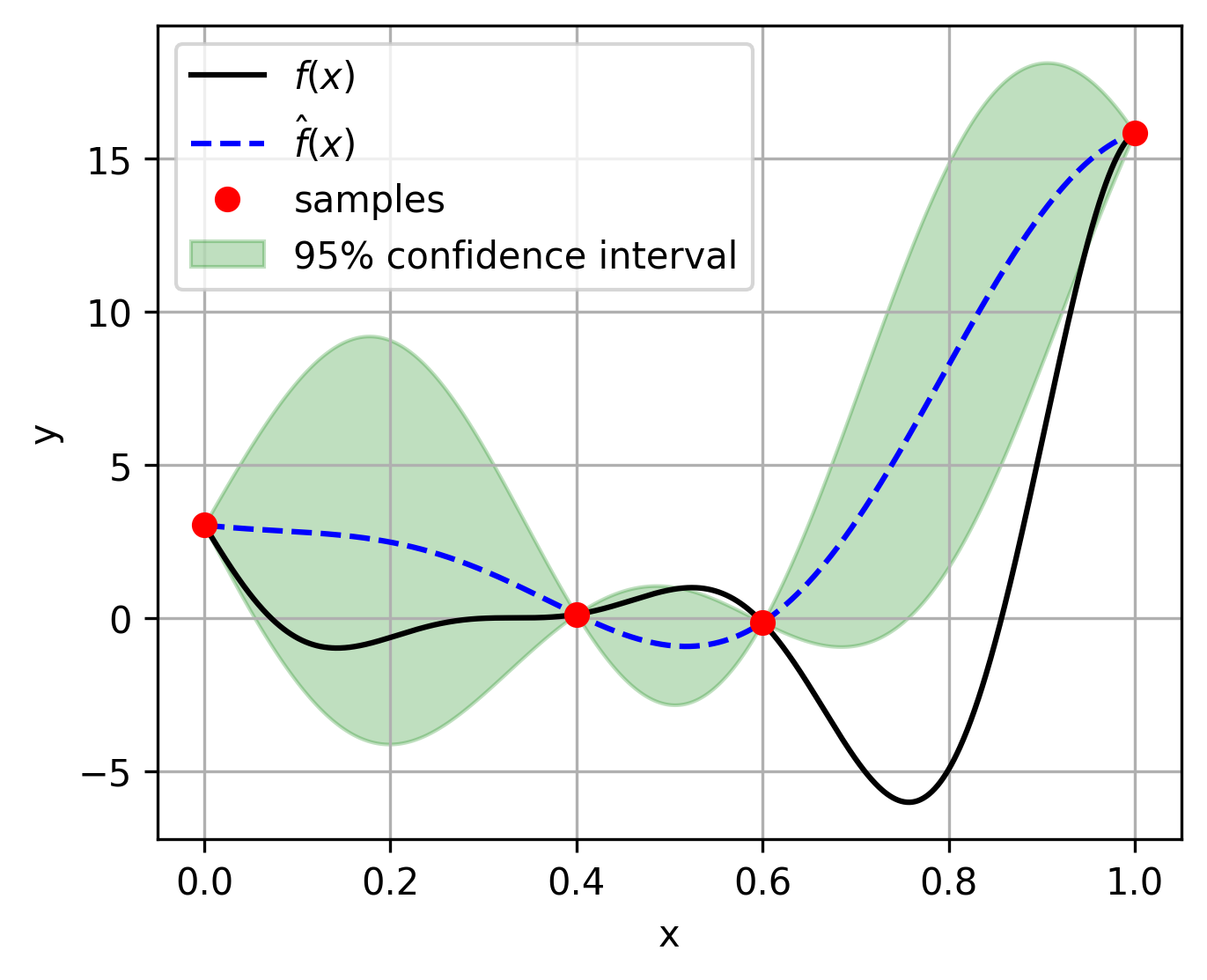
The Kriging model is implemented in GaussianProcessRegression class, where we have to assign noise_prior=0.0. The following example is given to illustrate the usage of the Kriging model:

# Import required libraries
import matplotlib.pyplot as plt
import numpy as np
from mfpml.models.gaussian_process import GaussianProcessRegression
from mfpml.problems.sf_functions import Forrester
from mfpml.models.basis_functions import Ordinary

# Define the target function
func = Forrester()

# Sample points for training
sample_x = np.array([0.0, 0.4, 0.6, 1.0]).reshape((-1, 1))
sample_y = func.f(sample_x)

# Generate test points
test_x = np.linspace(0, 1, 1001).reshape(-1, 1)
test_y = func.f(test_x)

# Initialize and train the Gaussian Process Regression model
model = GaussianProcessRegression(design_space=func.input_domain, regr=Ordinary(), noise_prior=0.0)
model.train(sample_x, sample_y)

# Make predictions
predictions, std_dev = model.predict(test_x, return_std=True)

# Plot the results
fig, ax = plt.subplots(figsize=(5, 4))
ax.plot(test_x, test_y, "k-", label=r"$f(x)$")                  # True function
ax.plot(test_x, predictions, "b--", label=r"$\hat{f}(x)$")      # Predicted function
ax.plot(sample_x, sample_y, "ro", label="Samples")              # Training samples
ax.fill_between(
    test_x.reshape(-1),
    (predictions - 1.96 * std_dev).reshape(-1),
    (predictions + 1.96 * std_dev).reshape(-1),
    color="g",
    alpha=0.25,
    label="95% confidence interval"
)
ax.legend(loc="best")
ax.set_xlabel("x")
ax.set_ylabel("y")
ax.grid()
plt.show()

Gaussian process regression for noisy data

1. basics of general Gaussian process regression

If we want to model a problem with noise within the outputs, where the problem can be formulated as:

\[y = f(x) + \epsilon\]

where \(\epsilon\) is the noise, which is assumed to be a Gaussian distribution with zero mean and variance \(\sigma_a^2\). Usually, this noise from data is called aleatory uncertainty, which is irreducible. So the general Gaussian process regression is proposed to model the aleatory uncertainty. The essence of the general Gaussian process regression is to model the noise as a white noise process, which is defined as:

\[k(\mathrm{x}, \mathrm{x}') = \sigma_a^2 \delta(\mathrm{x}, \mathrm{x}')\]

Intuitively, the white noise Correlation matrix is a diagonal matrix with diagonal elements \(\sigma_a^2\)

So the mix-kernel can be expressed as:

\[K_{mix}\left (\mathbf{X}, \mathbf{X} \right) =K_{RBF}\left (\mathbf{X}, \mathbf{X} \right) + K_{noise}\left (\mathbf{X}, \mathbf{X} \right)\]

Note

The general Gaussian process regression is implemented in GaussianProcessRegressor class. The hyper-parameter estimation and inference process of general Gaussian process regression model is the same as the Kriging model, just the correlation matrix is different. replace the original correlation matrix with the mix-kernel correlation matrix.

1. Implementation

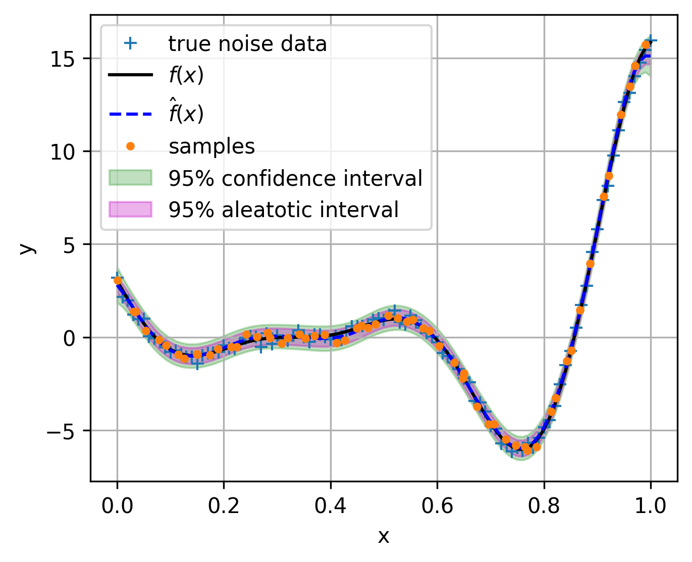
The general Gaussian process regression model is implemented in GaussianProcessRegressor class. The following example is given to illustrate the usage of the general Gaussian process regression model:

from mfpml.models.gaussian_process import GaussianProcessRegression
from mfpml.optimization.evolutionary_algorithms import DE
from mfpml.design_of_experiment.sf_samplers import LatinHyperCube

# sampling
sampler = LatinHyperCube(design_space=func._input_domain)
sample_x = sampler.get_samples(num_samples=30)
test_x = np.linspace(0, 1, 101, endpoint=True).reshape(-1, 1)

# get samples by adding noise to the true function
sample_y = func.f(sample_x) + np.random.normal(0, 0.2,
                                              sample_x.shape[0]).reshape((-1, 1))
test_y = func.f(test_x) + np.random.normal(0, 0.2,
                                          test_x.shape[0]).reshape((-1, 1))
test_mean = func.f(test_x)

# get samples by adding noise to the true function
sample_y = func.f(sample_x) + np.random.normal(0, 0.2,
                                              sample_x.shape[0]).reshape((-1, 1))
test_y = func.f(test_x) + np.random.normal(0, 0.2,
                                          test_x.shape[0]).reshape((-1, 1))
test_mean = func.f(test_x)

# initialize optimizer
optimizer = DE(num_gen=1000, num_pop=50, crossover_rate=0.5,
              strategy="DE/best/1/bin")
# initialize the regressor
gp_model = GaussianProcessRegression(
    design_space=func._input_domain, optimizer_restart=20, noise_prior=None)
# train the model
gp_model.train(sample_x, sample_y)
# get the prediction
sf_pre, sf_std = gp_model.predict(test_x, return_std=True)

# plot the results
fig, ax = plt.subplots(figsize=(5, 4))
ax.plot(test_x, test_y, "+", label="true noise data")
ax.plot(test_x, test_mean, "k-", label=r"$f(x)$")
ax.plot(test_x, sf_pre, "b--", label=r"$\hat{f}(x)$")
ax.plot(sample_x, sample_y, ".", label="samples")
ax.fill_between(
    test_x.reshape(-1),
    (sf_pre - 1.96 * sf_std).reshape(-1),
    (sf_pre + 1.96 * sf_std).reshape(-1),
    alpha=0.25,
    color="g",
    label="95% confidence interval",
)
ax.fill_between(
    test_x.reshape(-1),
    (sf_pre - 1.96 * gp_model.noise).reshape(-1),
    (sf_pre + 1.96 * gp_model.noise).reshape(-1),
    alpha=0.3,
    color="m",
    label="95% aleatotic interval",
)
ax.legend(loc="best")
ax.grid('--')
plt.xlabel("x")
plt.ylabel("y")
plt.savefig("general_gaussian_process_regression.png", dpi=300, bbox_inches="tight")
plt.show()